Building adb: Columnar Database System with PAX-style Page

December 26, 2024 07:20

When I was 10, I tried to create my own database. Of course, it’s nothing fancy. It’s just a system standing on top of the shoulder of Microsoft Access with Visual Basic 6.0 front-end. But last Fall 2024 I took Prof. Stratos’s class and, within 4 months, I developed my own multi-client, column-store database system, complete with a multi-threaded engine optimized to utilize all physical cores of the host system.

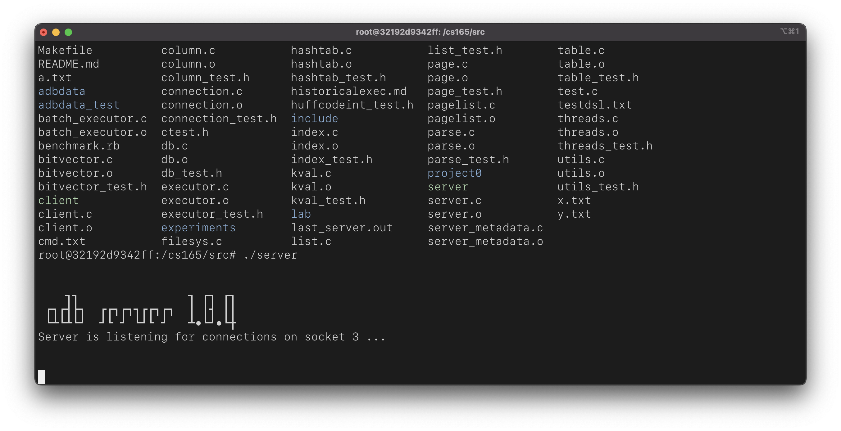
Look at this:

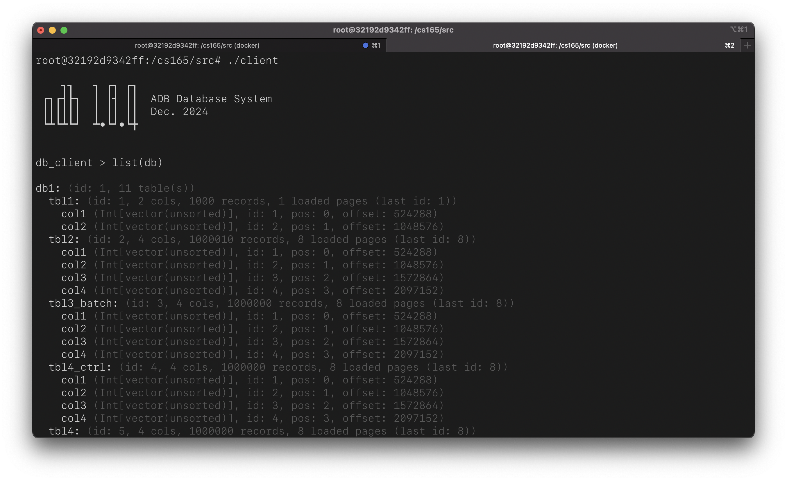
Then we can start a client app, and let’s list the database:

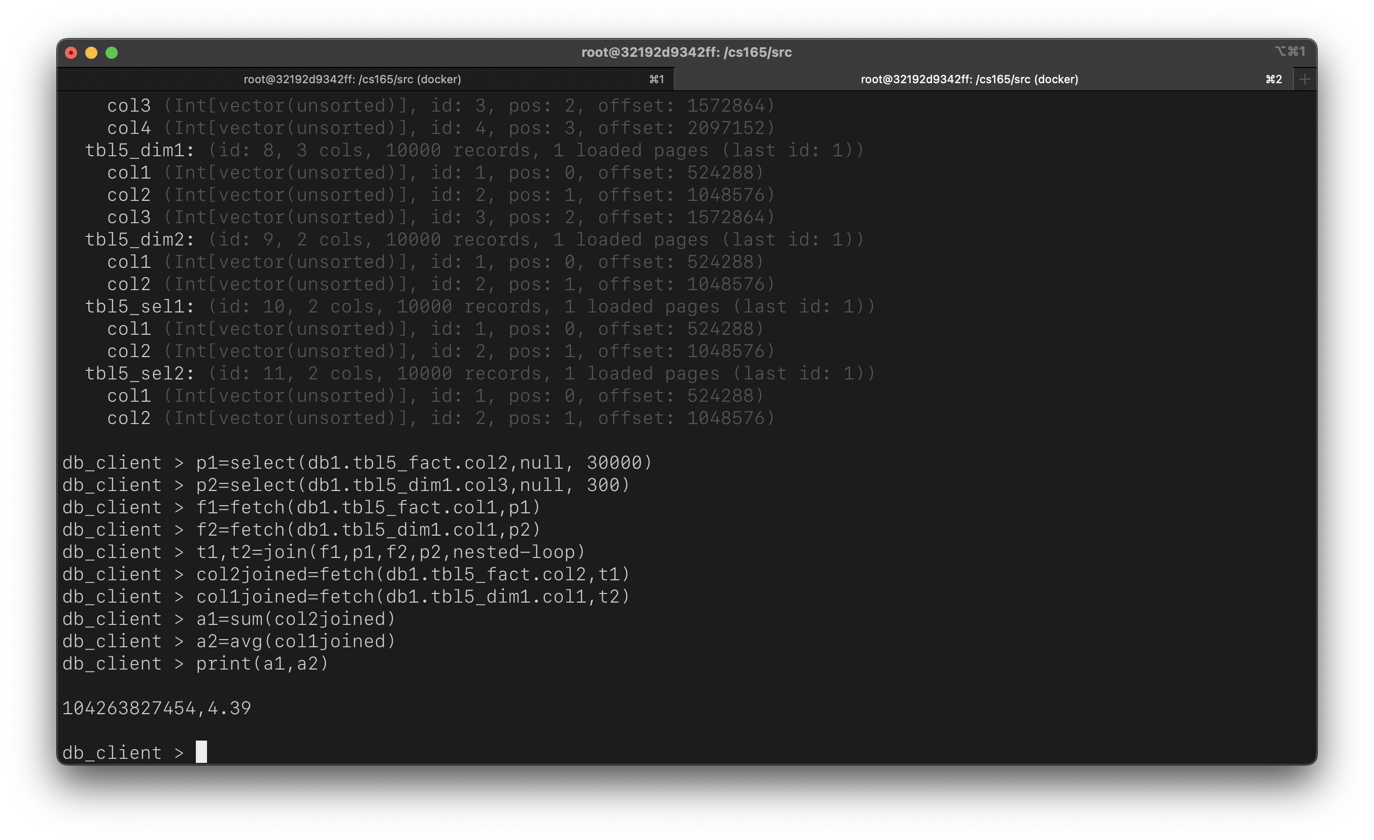
Let’s execute the following query to showcase the capability of adb:

SELECT sum(tbl5_fact.col2), avg(tbl5_dim1.col1)
FROM tbl5_fact, tbl5_dim1
WHERE tbl5_fact.col1 = tbl5_dim1.col1
AND tbl5_fact.col2 < 30000
AND tbl5_dim1.col3 < 300;

That is but a glimpse of what the system can do (and the amount of code that’s been written). In this document, I will detail my design decisions and reflect on areas where things could have been improved. Before diving deeper, it’s important to note that the system is built using plain, old C.

Database catalog

A database must have a catalog. In our case, this catalog records all the database and their columns, but not their rows. Before a shutdown, our database must persists the catalog or otherwise, upon restart, some databases or columns can be missing. In a way, therefore, this catalog enables users to persist the system’s state, enabling them to retain their previous databases and tables structure for future use.

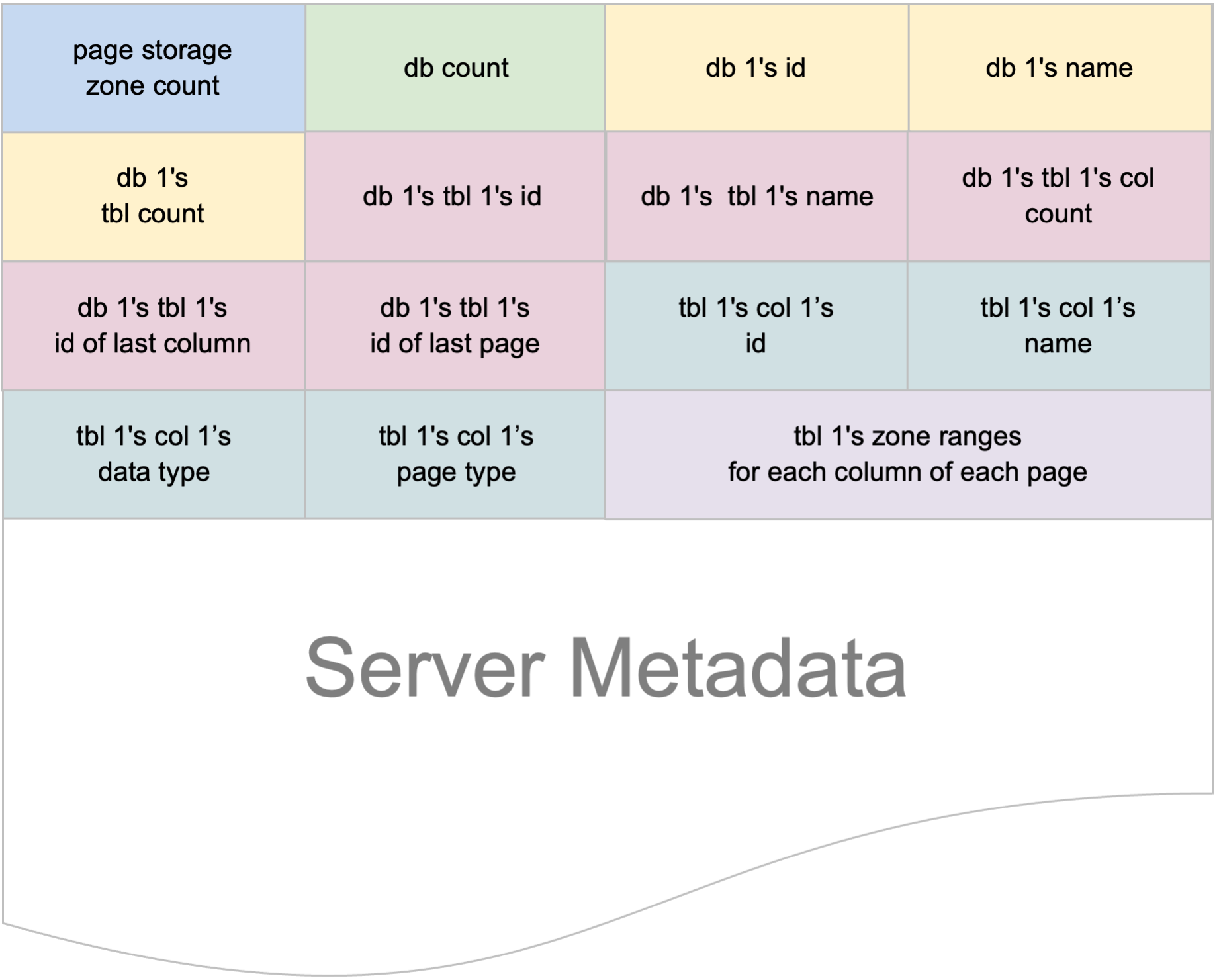
In our system, this is achieved by the ServerMetadata struct. As evident from the structure above, it primarily maintains the structure of all the tables in each database. We also record the number of database in the system, so that we can iterate all the database in the file correctly. This kind of counters also present for each database to record the number of columns in any given database. This is because our server metadata is a flat file, not JSON or the like.

Recording records and result set

We use a Page to store data for each column in a given table. A page has more or less the following structure. Notice that one single Page file has several columns in it, this design is inspired from PAX page.

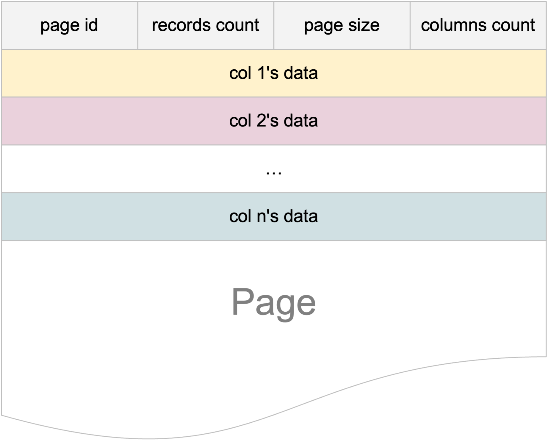
In actuality, Page is an overloaded concept: it can correspond to a table, or it may act as a result set for computation. When a Page corresponds to a table, it is disk-resident. The page file is created and opened if it doesn’t already exist, when we’re reading or writing values to any given column. Each page is formatted in a PAX-style, where columns are laid out in an offset one after another. Logically, we can write as much data to a column as needed, but physically, on a disk-resident Page, each Page has a maximum size limit. That is, if the page size is 2MB, it can store approximately 500,000 4-byte integers. If additional integers need to be stored, a new page is created and linked accordingly, with the system managing all necessary bookeeping as server metadata.

Conversely, when a Page acts as a result set, it lacks the ability to persist itself to a file. This kind of page is memory-resident, associated to a variable, such as illustrated from the following operation:

-- get positions of qualifying rows from db.tbl where grade is an int within the range of 70 to 100
a_plus = select(db.tbl.grade, 70, 100)

-- fetch the corresponding values
ids = fetch(db.tbl.student_id, a_plus)

In the case above, a Page associated to the ids variable holds data of the student_id column which pass the a_plus filter. For this use case, the Page holds only a single column’s data.

Meanwhile, the a_plus records qualifying record positions resulting from a select statement. For this, we use streams of bits, whereby the bit position represents the position of record. If the bit is turned on (1), then the record at that position qualifies a select statement. By doing so, instead of using 4 bytes, for instance, to record four qualifying positions, we can just use 1 byte (or char) since a char normally consists of 8 bits in most systems. This kind of data structure is called bit vector. That being said, a BitVector may not always be the optimal choice for representing positions such as if only the data at row 9,000 qualifies, we have to waste the other 8,999 bits. This, however, can be optimized, but our system doesn’t perform this kind of bit compression just yet.

How the BitVector and Page work together is that, on a given select statement, for example, if the table has 10 Page objects, we will then have 10 BitVector objects one for each Page, that is, the first BitVector represents qualifying positions on Page 1. But, when we translate those selection using fetch, the fetched data is stored in a single, continuous vector, no longer separated page by page. In summary, the result of a select is one BitVector for each Page of the table, whereby the result of a fetch is a flat vector of values in a memory-resident Page.

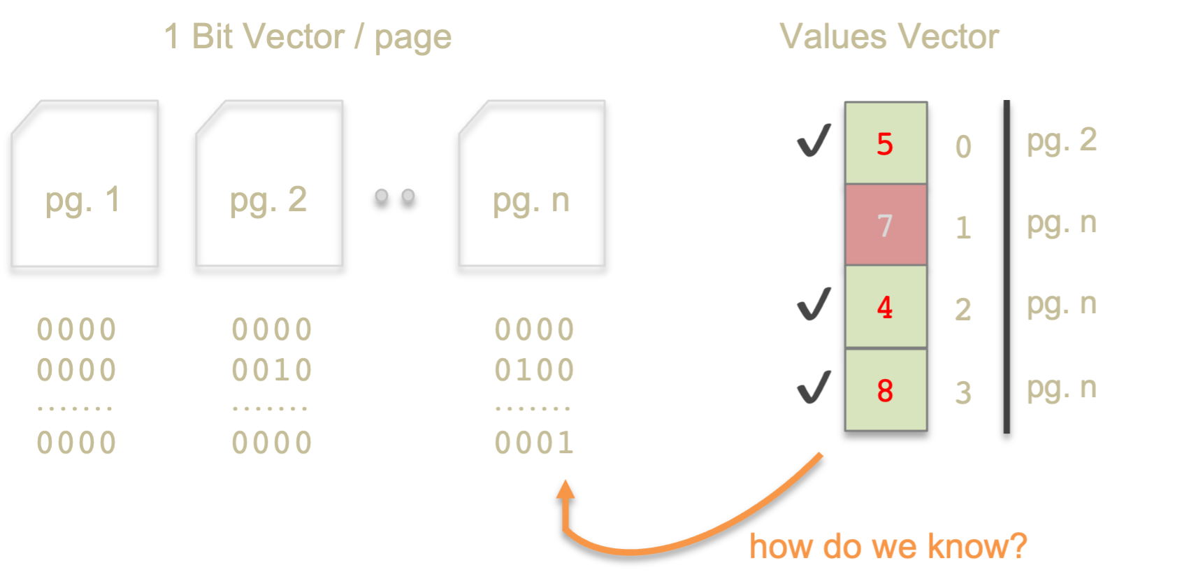
So, how can we utilize such configuration for further select and fetch, as essentially they are of different dimension? To imagine this problem better, assume that we have a state like the image above, where we have n-number of BitVector for each page, and a value vector containing 4 values from a previous fetch. The value vector has 5 at index 0 (fetched from page 2 at a certain position), 7 from page n, 4 at page n, and 8 at page n. In the eyes of the value vector, they are flat as in they have no information from which page and at which position they are mapped from. Now, to restate the question: how do they (BitVector and Page of different dimensions) know and relate each other?

You would imagine we invent a new data structure for bookkeeping, but that’s not necessary. The original intention of the BitVector data structure is to record as 1 each position in the column that satisfied a select criteria. This means, each 1 maps sequentially to each value in the values vector. Which means, every value not matching a future select can simply have those bits turned off (set to 0).

Perhaps, however, although this format might be one that is used in the industry, this PAX-style layout may be slower than a flat array structure where data is clumped together, forming a big chunk of array. With this structure, when we read a different page, the new page must be moved, however, they don’t form a contiguous chunk. The code below demonstrates how costly ineffective (or, non cache-conscious) data movement can be.

#include <sys/time.h>
#include <stdlib.h>
#include <stdio.h>
#include <string.h>


void cache_friendly_assignment(int** array, int dimension1_max, int dimension2_max) {
    printf("Using cache-friendly order\n");
    for (int i = 0; i < dimension1_max; i++) {
      for (int j = 0; j < dimension2_max; j++) {
        array[i][j] = 0;
      }
    }
}

void cache_unfriendly_assignment(int** array, int dimension1_max, int dimension2_max) {
    printf("Using cache-unfriendly order\n");
    for (int j = 0; j < dimension2_max; j++) {
      for (int i = 0; i < dimension1_max; i++) {
        array[i][j] = 0;
      }
    }
}

int main(int argc, char *argv[]) {
    printf("Experimenting with array traversal orders and cache friendliness.\n");

    int dimension1_max = 20000;
    int dimension2_max = 20000;
    int** array;

    array = malloc(dimension1_max * sizeof(int*));
    for (int i = 0; i < dimension1_max; i++) {
      array[i] = malloc(dimension2_max * sizeof(int));
    }

    struct timeval stop, start;
    gettimeofday(&start, NULL);

    if (argc != 2) {
      printf("expecting friendly or unfriendly as a parameters\n");
    }
    else if (strcmp(argv[1], "friendly") == 0) {
      cache_friendly_assignment(array, dimension1_max, dimension2_max);
    }
    else if (strcmp(argv[1], "unfriendly") == 0)  {
      cache_unfriendly_assignment(array, dimension1_max, dimension2_max);
    }
    else {
      printf("Did not get a valid parameter. Expecting friendly or unfriendly.\n");
    }

    gettimeofday(&stop, NULL);
    double secs = (double)(stop.tv_usec - start.tv_usec) / 1000000 + (double)(stop.tv_sec - start.tv_sec);
    printf("Execution took %f seconds\n", secs);

    for (int i = 0; i < dimension1_max; i++) {
      free(array[i]);
    }
    free(array);

    return 0;
}

Running the code above yields:

➜  lab git:(milestone-4) ✗ ./memhier friendly
Experimenting with array traversal orders and cache friendliness.
Using cache-friendly order
Execution took 0.668072 seconds
➜  lab git:(milestone-4) ✗ ./memhier unfriendly
Experimenting with array traversal orders and cache friendliness.
Using cache-unfriendly order
Execution took 3.526412 seconds

Why is the cache-unfriendly code so slow? Well, because we need to move data back and forth between the memory hierarchy where each level has varying speed. The video below is a great demo of speed different between the hierarchy.

Therefore, the following kind of code:

for (i = 0; i < n; i++) {
    min = a[i] < min ? a[i] : min
    max = b[i] > max ? b[i] : max
    // ...c, d, e
}

Would perform worse than the code below, because the code below doesn’t have random access as it moves data sequentially page by page:

for (i=0; i<n; i++) min = a[i] < min ? a[i] : min
for (i=0; i<n; i++) max = b[i] > max ? b[i] : max

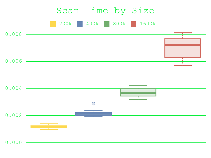
This is why, in the graph below, we observe greater variability in scan performance for larger datasets. This can be attributed to the fact that pages can be more easily evicted out of cache, if it’s full.

Unfortunately, with just four months to work (alongside a full-time job), there wasn’t much time to experiment with optimizing the system further. Cache-consciousness is only one factor to consider. For instance, it may seem counterintuitive, but sometimes reading or accessing data multiple times, shared over n number of queries, can be more efficient than reading it all at once—especially if we have a small TLB. Given more time, I would like to experiment with the following:

1. Data zoning: While I’ve implemented zones in the system, they weren’t utilized due to time constraints.
2. Zig-zag scanning: Instead of having five queries share data in a left-to-right scan (which may not be TLB-friendly), we could read a portion of the data, and then alternate reading left-to-right and right-to-left for each query. The goal would be to maximize the use of data already loaded in memory.

Managing variables

The a_plus and ids variable above need to be organized in such a way that each connected client have their own namespace to avoid naming clash. The Radix data structure is used, so instead of sequentially performing strcmp as in an array of string, we navigate down the tree substring by substring until reaching a node that corresponds to the key as a whole. Perhaps, however, it would be simpler and just as fast, if not better, to use hash table. Or, if we know that the number of variables wouldn’t be too much, we can as well just use an array. I feel, using Radix for this is pretty much an overengineering in terms of complexity, and at the end of the day, it might not result in a noticably faster lookup – if it’s even any faster. A study “A Comparison of Adapative Radix Trees and Hash Table” concludes that hash table can be significantly faster, and it’s not too hard to imagine way, since we just hash the key numerically once, and then go to a set of bucket, and simply scanning a flat, contiguous array from there. It has been said, and proven, that trees, indeed, may have similar performance as hash table, yet generally a tree is a harder data structure to implement in comparison to hash table. Not to mention, as we already discussed above, random access slow things down, and it seems that, it is much likely to have random access in a tree than in a hash table. Tree is worth it when there are large data stored in it, but if we just have only a few, the random access overhead can be too expensive.

Supporting multiple-clients

Multi-clients or multi-connections is probably one of the hardest to implement, so much that I was the only in my cohort to be able to successfully implement a multi-clients database system. The underlying idea is simply: when any client make a query to the server, the server will be able to recognize who’s who. So, it is necessary for each client to have their own context. The harder problem is implementing a reliable socket connection, since two clients/connections may send messages at the same time: how can you make sure that the pipeline is reliable, in that data is not smashed against one another? For this, we implement a Message struct, and a whole lot of studying of how networking socket works in a POSIX/UNIX-compliant system. It was arduous.

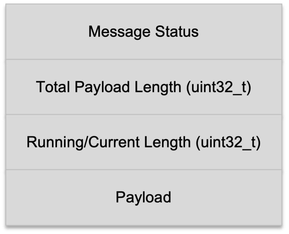
There are also many low-level cases to be dealt with, for example if a socket connection is terminated on one end, normally the other end will also terminate, so we must prevent this by setting the signal to MSG_NOSIGNAL and/or listening to EPIPE error. Such is just an example of the edge case to be dealt with.

How do we index data?

We support two types of indexing: clustered index, which roughly corresponds to the primary key, and unclustered index. Users are free to choose the underlying data structure for an index, be it sorted vector or B-Tree, yet the general principle remains the same: data will be sorted relative to the clustered index. In a sorted vector, data insertion and retrieval are facilitated by binary search. Important to note is that data is sorted independently for any unclustered indexes, where mapping to the original insertion position is maintained. Doing so allows us to resolve any data in the unclustered index to other columns in the table.

Let’s now create a database table with a clustered index, where the underlying storage structure is a B-Tree. We’ll also have an unclustered index where data is stored as a sorted vector. The query to create such a database table in our database looks like this:

create(tbl,"tbl4_clustered_btree",db1,4)
create(col,"col1",db1.tbl4_clustered_btree)
create(col,"col2",db1.tbl4_clustered_btree)
create(col,"col3",db1.tbl4_clustered_btree)
create(col,"col4",db1.tbl4_clustered_btree)
create(idx,db1.tbl4_clustered_btree.col3,btree,clustered)
create(idx,db1.tbl4_clustered_btree.col2,sorted,unclustered)

Our system took ~0.26s to run the two queries below on the tbl4_clustered_btree table pre-loaded with a million of records.

SELECT col1 FROM tbl4_clustered_btree WHERE col3 >= 44284 and col3 < 44484;

SELECT col1 FROM tbl4_clustered_btree WHERE col3 >= 167718 and col3 < 168118;

However, running a similar query against tbl4, which has no index, results in roughly the same runtime. Why is that? Why isn’t it slower, given that we’re using **no** index? Well, research has shown that when selectivity is high, using an index may not speed up the scan. This is what makes database systems so complex and fascinating! There are so many factors to consider and alternative approaches to explore, making it feel as-if the software is designed primarily to outsmart the hardware, instead of just as a data base.

How to do join?

There are some basic algorithms such as nested loop. Literally, in nested loop, we simply iterate result set from the left and match it with that on the right, one row at a time for each, and then note all matching rows.

new resL[]
new resR[]
k = 0
for (i = 0; i < L.size; i++)
  for (j = 0; j < R.size; j++)
    if L[i] == R[j]
      resL[k] = i
      resR[k++] = j

Hash join is another alternative that the system use. In hash join, inputs from either table are hashed, so they’ll be the sme if they match. There are many more advanced join algorithms such as grace hash, index join, sort merge, and others which we did not have the time to implement.

Conclusion

There is so much to explore and experiment with in this class. One of the most time-consuming and challenging tasks was implementing multi-client connectivity. In fact, I was the only one in the class to implement it “correctly” (meaning: it works, though I’m not sure how an “actually” correct implementation would look in a production system, but mine seems reasonable). It felt like a trade-off: either I could have used my time to implement other “core” features, like index joins, or I could focus on implementing “addons” like supporting multi-client connectivity. Regardless, I now have a better understanding of how to build a database system and have a deeper appreciation for its complexity, such that I understand the importance of hardware-software co-design in this field. Kudos to all database system developers. Anyway, you may also be interested in reading my literature review on NoSQL databases.