Building a Movie Recommender using Autoencoder
August 17, 2024 18:10
In the old days, one would require a rather serious statistical analysis to come up with a single recommendation system, such as by using basket of items and group together items in any given basket that occur too many times together on different occasions. The development of such a system is very resource-intensive, and easily out of reach without adequate statistical knowledge. Nowadays, Artificial Intelligence has advanced so much that there could be no need for such a deep, manual work. One would be able to come up with 4 different recommendation systems within a day by using artificial intelligence.
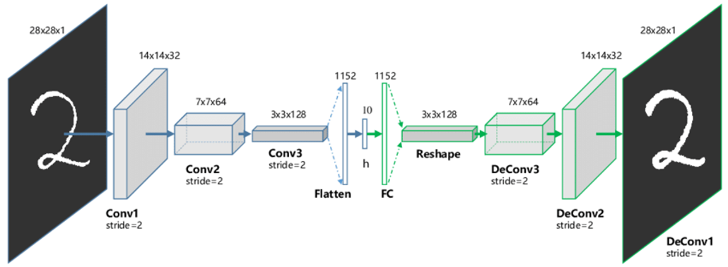
To that end, we will use autoencoder, which is renowned for its feature extraction capabilities, among other functions. Unlike other neural network architectures, the output node in an autoencoder is not open-ended; instead, it is connected to a decoder, which consists of multiple layers of neurons. During training, the network is fed a dataset 𝑥 and is tasked with predicting this same, exact dataset.
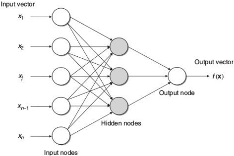
The constant feeding of an autoencoder’s own input to predict itself results in the “output” node experiencing what is known as dimensionality reduction. This is particularly evident in the use of an undercomplete autoencoder, where the “output” node is significantly smaller than both the encoder and the decoder. At this stage, it is more accurate to refer to this “output” node as the latent space or the coding. The presence of this latent space is a unique characteristic of an autoencoder. Essentially, an autoencoder is a neural network that attempts to replicate its input in such a way that it does not merely memorize the data. This ability prevents it from simply duplicating the input and enables it to perform creative tasks such as noise removal and music generation. This preference for an undercomplete autoencoder is due to its non-linear transformation, which ensures that the network does not produce identical reconstructions of the input. After all, it is not so interesting if our recommendation system recommended pretty much the same exact movies the user has already watched.
Throughout this experiment, I use Azure AI Machine Learning Studio, it was great! I can use nVidia A100 at all time I need it. That aside, the packages that I use are:
- Python 3.9.19
- Keras 3.4.1
- Pandas 2.2.2
- Numpy 1.26.4
- Matplotlib 3.9.1
Our dataset comes from a research by GroupLens Research, which collected and made available movies rating data set. To download it, go to their website , look on MovieLens 32M, download ml-32m.zip, which was collected on 10/2023 and released on 05/2024.
In that zip file, there are two files of utmost interest for us:
- ratings.csv
- movies.csv
The rating data set consists of each user’s rating of a movie. The smallest rating given by anyone is 0.5, whereby 5.0 is the maximum rating. In total, there are no less than 32 billion ratings for any of the 87,585 movies. The ratings.csv file looks like this:
| user_id | movie_id | rating |
|---|---|---|
| 1 | 17 | 4 |
| 1 | 25 | 1 |
| 1 | 29 | 2 |
Interestingly, although there is no missing data (i.e., “nan”), the movie IDs are not sequential, despite being entirely numerical. This is important to note because, represented as a matrix, we must carefully represent it so that each row represents a user and each column a movie. Given that in any matrix of size 𝑚 × 𝑛, the columns are sequentially numbered from 0 to 𝑛, non-sequential movie IDs cannot be naively mapped to matrix columns without careful handling.
Modeling and Training
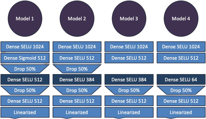
We will have 4 different models for training and prediction, of which their architecture are summarized as follows:
Or, in code:
model1 = models.Sequential([
    layers.Input(shape=inter_matrix.shape[1:]),
    layers.Dense(1024, activation="selu"),
    layers.Dense(512, activation="sigmoid"),
    layers.Dropout(0.5),
    layers.Dense(512, activation="selu", name="coding"),
    layers.Dropout(0.5),
    layers.Dense(512, activation="selu"),
    layers.Dense(inter_matrix.shape[1], activation="linear", name="score_pred")
])

model2 = models.Sequential([
    layers.Input(shape=inter_matrix.shape[1:]),
    layers.Dense(1024, activation="selu"),
    layers.Dense(512, activation="selu"),
    layers.Dropout(0.5),
    layers.Dense(384, activation="selu", name="coding"),
    layers.Dropout(0.5),
    layers.Dense(512, activation="selu"),
    layers.Dense(inter_matrix.shape[1], activation="linear", name="score_pred")
])

model3 = models.Sequential([
    layers.Input(shape=inter_matrix.shape[1:]),
    layers.Dense(1024, activation="selu"),
    layers.Dense(512, activation="selu"),
    layers.Dense(384, activation="selu", name="coding"),
    layers.Dropout(0.5),
    layers.Dense(512, activation="selu"),
    layers.Dense(inter_matrix.shape[1], activation="linear", name="score_pred")
])

model4 = models.Sequential([
    layers.Input(shape=inter_matrix.shape[1:]),
    layers.Dense(1024, activation="selu"),
    layers.Dense(512, activation="selu"),
    layers.Dense(64, activation="selu", name="coding"),
    layers.Dropout(0.5),
    layers.Dense(512, activation="selu"),
    layers.Dense(inter_matrix.shape[1], activation="linear", name="score_pred")
])
For training, each model’s compilation hyperparameters is as follow:
| Model | Optimizer | Loss | Metrics |
|---|---|---|---|
| Model 1 | Adam, lr = 0.0001 | MSE | MAE, MSE, R2 |
| Model 2 | Adam, lr = 0.0001 | MSE | MAE, MSE, R2 |
| Model 3 | Adam, lr = 0.001 | MSE | MAE, MSE, R2 |
| Model 4 | Adam, lr = 0.001 | MSE | MAE, MSE, R2 |
Since our model is not for classification, but regression, using accuracy as metrics would be meaningless. Instead, as shown, we measure our model’s accuracy performance by using 4 different metrics: R2, MAE, MSE. Whereby, their training, or fitting hyperparameters are as follow:
| Model | x | Epochs | Validation data |
|---|---|---|---|
| Model 1 | 80% of 10% of data, in batch of 512 items | 30 | 20% of 10% of data, batch: idem |
| Model 2 | 80% of 10% of data, in batch of 256 items | 30 | 20% of 10% of data, batch: idem |
| Model 3 | 80% of 10% of data, in batch of 256 items | 30 | 20% of 10% of data, batch: idem |
| Model 4 | 80% of 10% of data, in batch of 256 items | 30 | 20% of 10% of data, batch: idem |
The form of the data we fed into each model is an interaction matrix, which could be created by pivoting the rating data frame in this way:
inter_matrix = ratings_df.pivot(
    index="user_id",
    columns="movie_id",
    values="rating"
)
However, doing so could be greatly costly if not outright impossible to do in most machines (without any other external tools). One way to make this pivoting possible is by manually creating a matrix, instead of a data frame.
def create_interaction_matrix():
    ratings = ratings_df.to_numpy()

    # extract rows and columns
    rows, row_pos = np.unique(ratings[:, 0], return_inverse=True)
    cols, col_pos = np.unique(ratings[:, 1], return_inverse=True)

    # pivot
    pivot_table = np.zeros((len(rows), len(cols)), dtype=ratings.dtype)
    pivot_table[row_pos, col_pos] = ratings[:, 2]

    # ensure all movies ever recorded are represented
    assert pivot_table.shape[1] == len(ratings_df['movie_id'].unique())

    # create the interaction matrix
    inter_matrix=pd.DataFrame(
        data=pivot_table[0:,0:],
        index=[i for i in range(pivot_table.shape[0])],
        columns=[i for i in range(pivot_table.shape[1])]
    )
    inter_matrix['user_id'] = ratings_df['user_id'].unique()
    inter_matrix.set_index('user_id', inplace=True)

    return inter_matrix
With the interaction matrix at hand, the training involves feeding the network with it in batches. Doing so prevents sending too much data into the GPU at once. This way, we can scale our training in case we want to train our network with 40%, instead of 10%, of data. But, in the result section, we will show off that training with just 10% of the interaction matrix can still yield a satisfying result.
Training
Upon training, we charted each model on a cartesian plane detailing their R2, MSE, and MAE score during the training. It is very interesting that Model 1 exhibits a significant gap between training and validation metrics in all measures during the initial stages of training. However, this gap diminishes as training progresses.
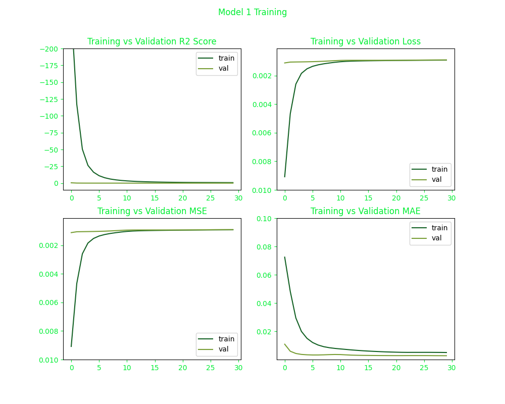
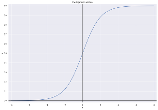
This observation can be attributed to the use of the sigmoid activation function in one of the encoder layers of this model. The sigmoid function, commonly denoted as σ(x) is mathematically defined as f(x) = 1 / (1 + e-x). This sigmoid function squashes its real-valued input to a value between 0 and 1 on the y-axis. As the sigmoid function asymptotically approaches 0 for large negative inputs and 1 for large positive inputs, it effectively normalizes the output of each neuron. This is why sigmoid is used a lot in models where we have to predict the binary probability of an output as a yes or a no. Another interesting characteristic is how it has a smooth gradient which prevents jumps in output values.
The sigmoidal characteristics of the activation function may contribute to Model 1 producing lower scores for each movie it recommends compared to the other models. This observation suggests that direct comparisons of scores between different models may be inherently flawed. For a more comprehensive evaluation, the training histories of the other models are presented as follows:
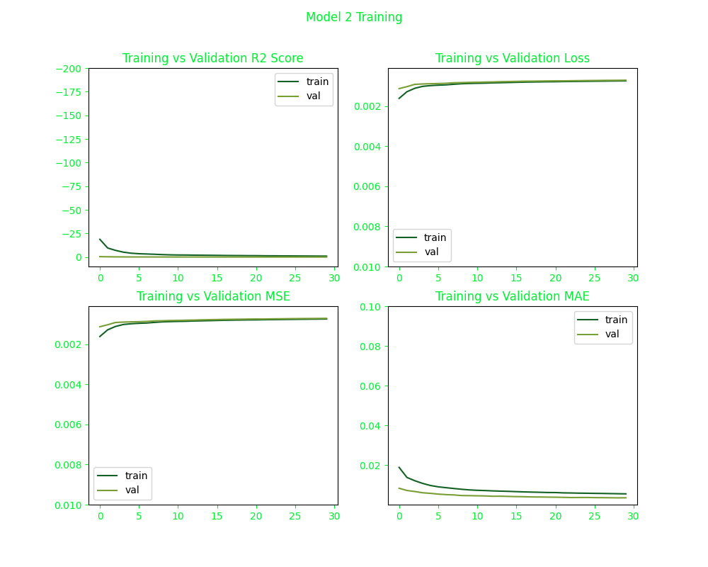
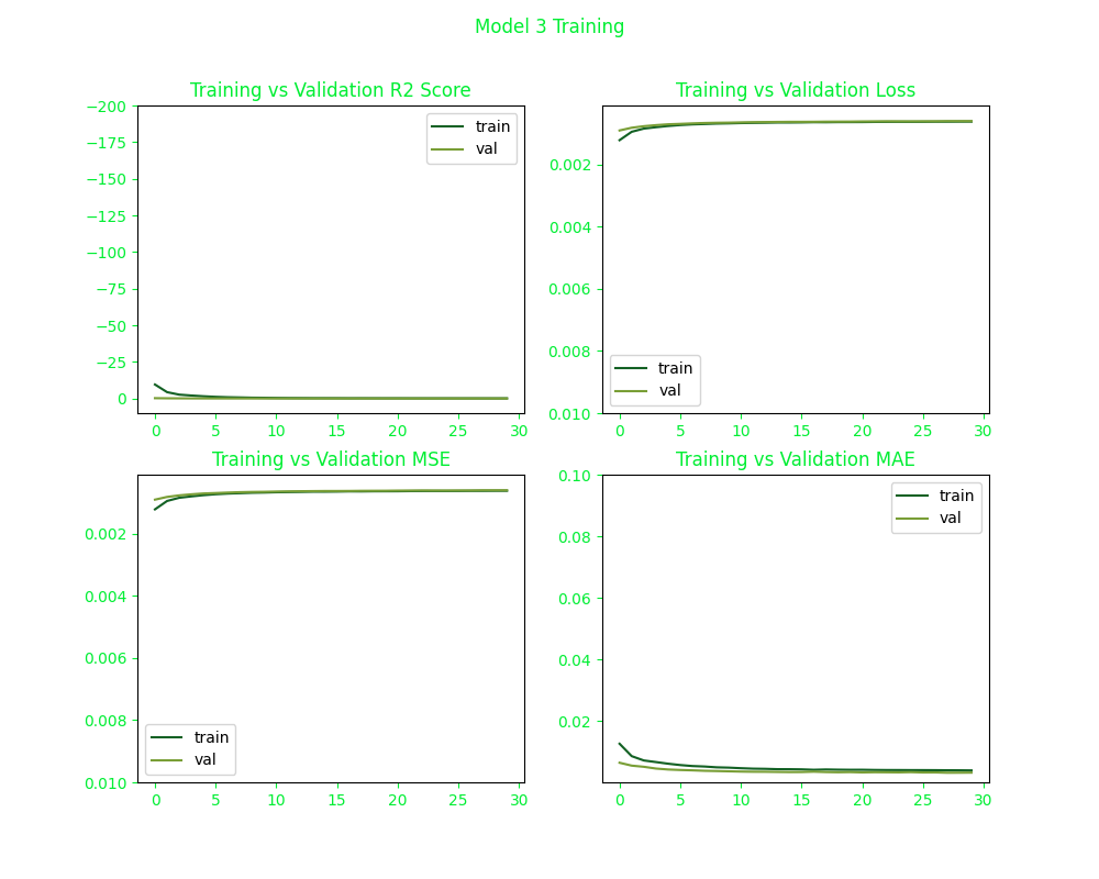
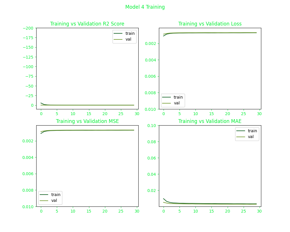
The impact of the SELU activation function is evident in the graphs, as it facilitates internal self-normalization of its inputs, potentially enabling the model to converge more rapidly without relying on batch normalization. In contrast, the use of the sigmoid activation function may be considered less optimal in this context. While sigmoid functions have traditionally been employed for classification works, along with hyperbolic tangent and softmax, their use in this case is somewhat controversial, although it’s true that historically, sigmoid were more commonly used before the advent of advanced techniques such as the Adam optimizer or He/Xavier initialization.
Yet, although our model is not designed for binary classification, we reason that employing the sigmoid activation function in the early layers of the encoder could be beneficial. This is because the sigmoid function, which maps outputs to a range between 0 and 1, can effectively indicate binary distinctions whether a movie is likeable or not. While sigmoid functions are traditionally used for binary classification tasks to produce outputs that reflect probabilities between 0 (no) and 1 (yes), in our case, we utilize it in the early layers to enhance the model’s ability to differentiate strongly between the likeability in this normalized range. In short, we liken what we do to something similar to market basket analysis, although this will need further research or proof to be certain of.
Result
To see our model predictions in practice, we will start with removing rated movies from the matrix. This can be achieved by running the following code.
model1_predictions = model1.predict(x) * (x == 0)
model2_predictions = model2.predict(x) * (x == 0)
model3_predictions = model3.predict(x) * (x == 0)
model4_predictions = model4.predict(x) * (x == 0)
With that code, if a User ID 10 has rated movies with the following IDs: 2, 3, 4, and 5, the above code will “remove” those movie IDs entirely to become:
| user_id | 1 | 6 | 7 |
|---|---|---|---|
| 10 | 0.509804 | 0.402111 | 0.398102 |
But that “removal” is only for a User ID 10, as another user, let’s say with ID 11 may have the following frame instead, for example.
| user_id | 6 | 7 | 11 |
|---|---|---|---|
| 11 | 0.020033 | 0.000925 | 0.003458 |
In short, we will see what kind of movies each model would recommend that any given user has never ever watched before. To touch base, these are the Top 7 movies rated by User ID 10.
| Score | Title | Genre/Theme | Release |
|---|---|---|---|
| 100% | Godfather, The | Crime, Drama | 1972 |
| 100% | Silence of the Lambs, The | Crime, Horror, Thriller | 1991 |
| 90.20% | Shining, The | Horror | 1980 |
| 90.20% | Fifth Element, The | Action, Adventure, Comedy, Sci-Fi | 1997 |
| 90.20% | Fear and Loathing in Las Vegas | Adventure, Comedy, Drama | 1998 |
| 90.20% | Exorcist, The | Horror, Mystery | 1973 |
| 90.20% | Star Wars: Episode V – The Empire Strikes Back | Action, Adventure, Sci-Fi | 1980 |
The Top 7 movies recommended by Model 1 includes the following:
| Score | Title | Genre/Theme | Release |
|---|---|---|---|
| 44.45% | American Beauty | Drama, Romance | 1999 |
| 39.66% | Fargo | Comedy, Crime, Drama, Thriller | 1996 |
| 36.78% | Good Will Hunting | Drama, Romance | 1987 |
| 35.16% | Monty Python and the Holy Grail | Adventure, Comedy, Fantasy | 1975 |
| 34.18% | Groundhog Day | Comedy, Fantasy, Romance | 1993 |
| 33.09% | Princess Bride, The | Action, Adventure, Comedy, Fantasy, Romance | 1987 |
| 32.43% | One Flew Over the Cuckoo’s Nest | Drama | 1975 |
It is difficult to argue that the model’s predictions are quite intriguing. For instance, Good Will Hunting is a compelling recommendation for individuals who enjoy drama and have also watched some science fiction, as the film’s narrative involves a janitor named Will Hunting whose mathematical prowess attracts the attention of an MIT professor, initiating a dramatic story. Similarly, titles such as Monty Python and Fargo, among others on the list, would likely resonate with User ID 10 in a similar manner.
Model 2 on the other hand, recommended the following top 7 movies:
| Score | Title | Genre/Theme | Release |
|---|---|---|---|
| 60.56% | Cantante, El | Drama, Musical | 2007 |
| 57.53% | Incredibles, The | Action, Adventure, Animation, Children, Comedy | 2004 |
| 53.06% | Monsters, Inc. | Adventure, Animation, Children, Comedy, Fantasy | 2001 |
| 47.54% | Green Mile, The | Crime, Drama | 1999 |
| 47.46% | Snatch | Comedy, Crime, Thriller | 2000 |
| 47.06% | Shaun of the Dead | Comedy, Horror | 2004 |
| 46.44% | Beautiful Mind, A | Drama, Romance | 2001 |
Meanwhile, Model 3 would recommend:
| Score | Title | Genre/Theme | Release |
|---|---|---|---|
| 52.15% | Beautiful Mind, A | Drama, Romance | 2001 |
| 42.73% | Maisie Gets Her Man | Comedy, Romance | 1942 |
| 42.03% | Cantante, El | Drama, Musical | 2007 |
| 41.44% | Charlie and the Chocolate Factory | Adventure, Children, Comedy, Fantasy, IMAX | 2005 |
| 41.38% | Bad Boys | Action, Comedy, Crime, Drama, Thriller | 1995 |
| 41.27% | Italian Job, The | Action, Crime | 2003 |
| 40.72% | Pandora’s Box (Pandora’nin kutusu) | Drama | 2008 |
Examining only the top seven recommendations reveals that Model 2 and Model 3 offer relatively broad suggestions. For instance, while WALL-E is categorized under Adventure and Sci-Fi, it differs significantly from Star Wars V and does not align with the adventurous and playful nature of Fear and Loathing in Las Vegas. However, restricting the analysis to just the top seven recommendations can be misleading. In reality, User 10 has demonstrated just as relatively strong preference for movies like Ice Age, The Lion King, E.T. the Extra-Terrestrial, and The Chronicles of Narnia.
Now, last but not least, our Model 4 would recommend the following movies:
| Score | Title | Genre/Theme | Release |
|---|---|---|---|
| 54.61% | Cantante, El | Drama, Musical | 2007 |
| 45.41% | True Lies | Action, Adventure, Comedy, Romance, Thriller | 1994 |
| 42.56% | Léon: The Professional (a.k.a. The Professional) (Léon) | Action, Crime, Drama, Thriller | 1994 |
| 41.13% | Agency | Drama | 1980 |
| 40.80% | Shaun of the Dead | Comedy, Horror | 2004 |
| 38.73% | Next Three Days, The | Crime, Drama, Romance, Thriller | 2010 |
| 38.04% | Bikini Summer | Comedy | 1991 |
By this point, it can be argued that Model 1 delivers more relevant predictions. The movies it suggests appear to capture latent variables, such as the release date, which are not even identified in our training, and so sorely missed by other recommendation models. Effectively, Model 1 infers that User 10 may have a preference for films from the 1960s, leading to recommendations that align with his taste but still conforming to the year dimension. Interestingly, Model 4 shares similarities with Model 1 while also including newer movies of the same genre from subsequent years. The absence of additional Star Wars recommendations might initially seem surprising; however, this is attributable to the fact that User 10 has already viewed nearly every film in the Star Wars franchise.
Determining which model is superior is inherently subjective and may vary depending on individual user preferences. For production use, it might be proper to use multiple models such that movies recommended by Model 1 and Model 4 should show up more, yet we will also have some movies fetched off from Model 2’s and Model 3’s data frame. Regardless, our experiment proves that we can use autoencoder to come up with a clever recommendation system in a day.
Pros and Cons
With this technique, the pros are:
- Quickly build recommendation systems in a day
- Can skip specific statistical theories such as market basket analysis
- Easy to tune the model’s behavior
Meanwhile, the cons:
- Can be hard to understand why it works the way it is
- Need training data, can’t start empty-handed
- Need retraining for new movies and rating data